Simulate survey

library(virtualecologist)

1. Generate a transect design

This design can be done with the dssd package when working on real-world examples.

The generate_survey_plan() function presented here provide facilities to build a simple layout. The built layout will consist of parallel transects covering a given area in the virtual environment, spaced out by a given distance and segmented by a given length. The layout can either be horizontal (the default) or vertical. The design can be generated in virtual or real space, but in the latter case, be cautious about the units (you should work with projected coordinates).

surv <- generate_survey_plan(bbx_xmin = 30, bbx_xmax = 65, bbx_ymin = 30, bbx_ymax = 65,
                             start_x = 34, end_x = 60, start_y = 34, end_y = 68,
                             space_out_factor = 2, segmentize = TRUE, seg_length = 1,
                             buffer = TRUE, buffer_width = 0.2)
par(mfrow = c(2,2), mar = c(2.5,2.5,4,0.5))
raster::plot(surv$bbx, axes = TRUE, main = "bounding box")
plot(sf::st_geometry(surv$transects), axes = TRUE, main = "transects")
plot(sf::st_geometry(surv$segments), axes = TRUE, main = "segments")
plot(sf::st_geometry(surv$buffered_segments), axes = TRUE, main = "buffered seg")

2. Assign a flight plan to the survey

Before launching a survey, a flight plan must be set up, that is the order by which segments will be surveyed must be chosen. This is done with assign_flight_plan(), which gets a segment objects (buffered segments from above), a vector providing the order by which segment table rows will be surveyed, the survey starting date and time, the speed of the aircraft (from which is calculated the survey duration of a single segment) and the duration of the transit period between two successive transects. The function automatically adds a one-second gap between two consecutive segments to avoid overlapping periods.

surv <- generate_survey_plan(bbx_xmin = 30, bbx_xmax = 65, bbx_ymin = 30, bbx_ymax = 65,
                             start_x = 34, end_x = 60, start_y = 34, end_y = 68,
                             space_out_factor = 2, segmentize = TRUE, seg_length = 1,
                             buffer = TRUE, buffer_width = 0.2
)


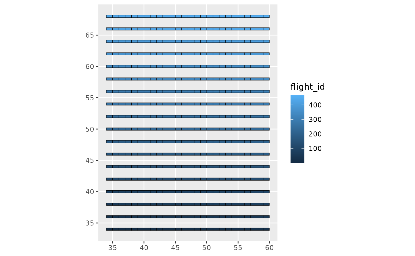
# assign the time periods to each segment
flight_plan <- assign_flight_plan(
  sf_segments = surv$buffered_segments,
  flight_id = c(1:468),
  col_trans_id = "transect",
  flight_day = "2022-08-01",
  survey_start_hour = "06:00:00",
  flight_speed = 160,
  intertransect_gap_duration = 60*30
)

# plot to check everything is ok
library(ggplot2)
ggplot(flight_plan) +
    geom_sf(aes(fill = start_time),
            color = "black", size = 0.2) +
    scale_fill_datetime(low = "#8073ac", high = "#fdb863") +
    theme_bw() + theme(panel.grid = element_blank()) +
    labs(fill = "Hour", limits = c("06:00", "16:16"), x = "x", y = "y")+
    coord_sf(xlim = c(0,90), ylim = c(0,90))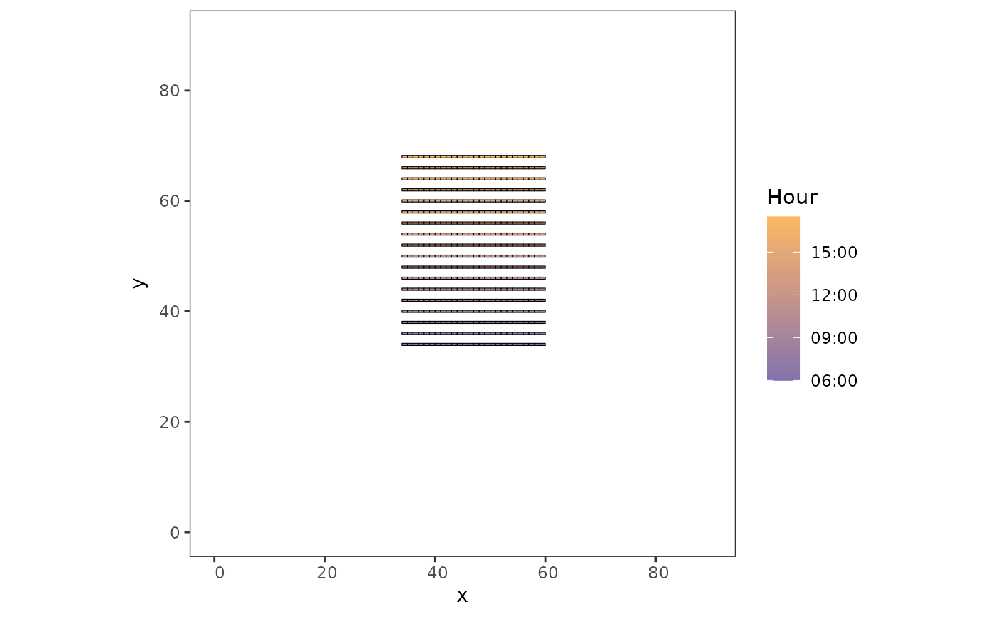

ggplot(flight_plan) +
    geom_sf(aes(fill = flight_id),
            color = "black", size = 0.2)

3. Simulate survey on fixed individual

The detection_process() function can be used to simulate the detection process when the surveyed individuals are fixed on the geographical space, for example when the species distribution is generated by simul_spat(). If strip_transect is emulated, an individual is considered detected if its distance to the track line is lower than the width (provided with sigma). If line-transect is emulated, a half-normal detection function is built using the given sigma as effective strip half-width. The user must define if the simulation is done in a virtual space or not (if not, the distances must be provided in km and pts and transects objects must be projected).

grid <- create_grid()
env <- generate_env_layer(grid = grid)
#> [using unconditional Gaussian simulation]
sp <- suppressWarnings(simul_spat(ref_map = env$rasters$sim1,
                 N = 1000, 
                 n_sim = 1, 
                 return_wgs_coordinates = FALSE))

pts <- detection_process(pts = sp, 
                         transects = example_data$survey$segments, 
                         strip_transect = TRUE, 
                         sigma = 0.2, 
                         virtual_space = TRUE,
                         seg_id_col = "seg_id")
#> Strip-transect is used with a width of 0.2
plot(sp$x, sp$y)
plot(sf::st_geometry(example_data$survey$segments), col = "red", add = TRUE)
points(sf::st_drop_geometry(pts[which(pts$detected == 1), c("x", "y")]), 
       pch = 20, col = "blue")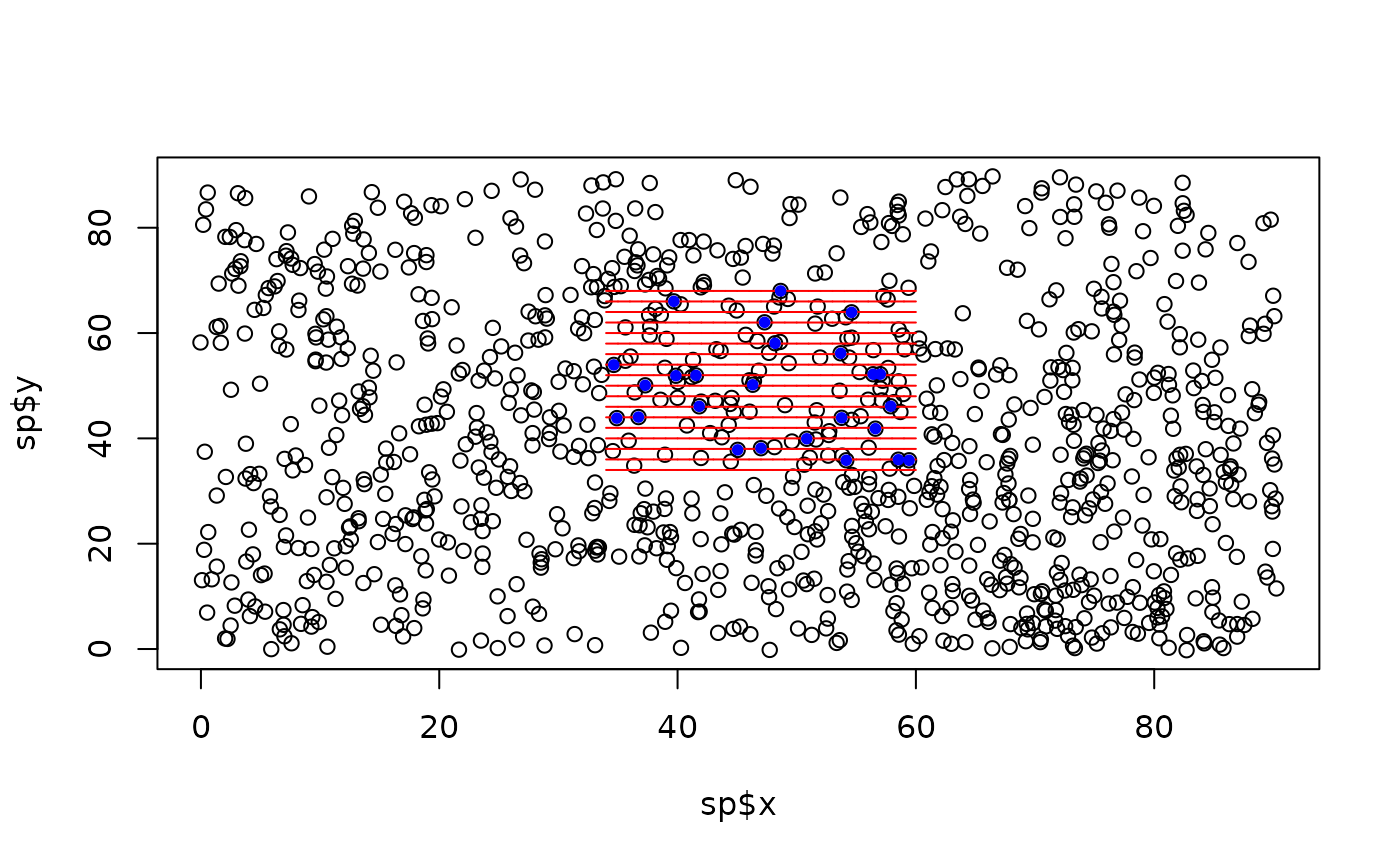

4. Simulate survey on moving individuals

Once we have the movements of a population on one hand, and a survey design with time periods assigned on the other hand, we can match the two to simulate the conduction of an observation survey. This is what is done by the launch_survey_on_movement() function, scrutinizing whether movement bouts temporally matching segments are included within them. If yes, and the centroid of the movement bout is included in the segment, the individual is considered as sighted by the survey. This default strip-transect protocol can be changed to line-transect protocol, in which case a distance-dependent detection probability is additionally computed for each individual as to defined whether or not they are detected during the survey.

For the survey to be relevant, the size of the buffer around the segments must be carefully chosen in generate_survey_plan() as to mimic the maximum distance to the track line considered possible during a survey (e.g. 200 m for a strip-transect survey; 1 km for a line-transect survey).

Note: there must not be a too large difference between the size of segments and that of movement bouts. Because the function simplifies the movement bouts to their centroids, movement bouts should be on the same time scale as the segments (seconds). Otherwise, the position approximated to define if the individual is sighted or not (i.e., the center of the movement bout) may not be representative of the movement of the individual.

# an example with a small number of individuals
survey <- launch_survey_on_movement(
  survey_data_buffered = example_data$flight_plan,
  survey_data_linear = example_data$survey$segments,
  traj_data = example_data$mvmt_data,
  line_transect = TRUE, detection_function = "hn",
  sigma = 0.2
)
#> Applying detection function

# look at the number of sightings
summary(survey$effort_table$N_ind_tot)
#>    Min. 1st Qu.  Median    Mean 3rd Qu.    Max. 
#> 0.00000 0.00000 0.00000 0.03846 0.00000 6.00000

plot(sf::st_drop_geometry(survey$obs_table[, c("dist_seg", "prob_dist")]), 
     xlab = "distance to the track line", ylab = "detection probability")

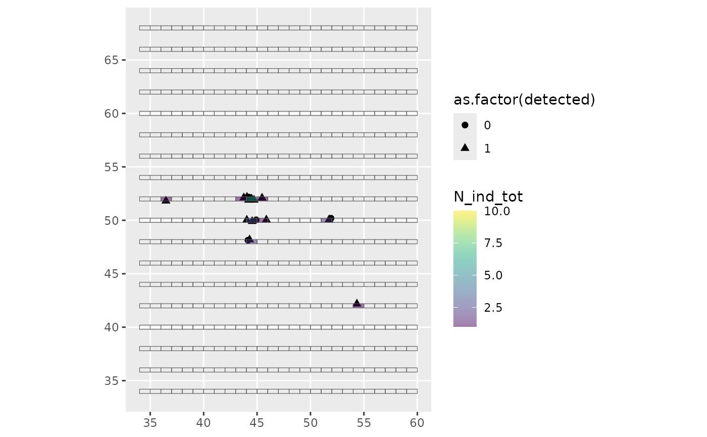
# all sightings are in a few segments
library(ggplot2)
ggplot(survey$effort_table) +
  geom_sf(data = survey$obs_table, 
          aes(shape = as.factor(detected)), size = 2) +
  geom_sf(aes(fill = N_ind_tot)) + 
  viridis::scale_fill_viridis(limits = c(1,10), 
                              na.value = NA, alpha = 0.5)