Simulate virtual environment • virtualecologist

library(virtualecologist)

Create the grid

Create the grid structuring the virtual environment. By default, create_grid() creates a grid spanning 0 to 90° in both longitude and latitude, with steps of 0.5.

grid <- create_grid()

Generating environmental layers

The generate_env_layer() function creates several environmental layers using Gaussian simulation from the grid locations. The number of layers generated is set by n. The generated layers can be normalised, and be returned either only as data frame or both in data frame and raster formats (SpatRast).

grid <- create_grid()

str(generate_env_layer(norm = FALSE, return_rasters = FALSE, grid = grid))
#> [using unconditional Gaussian simulation]
#> 'data.frame':    32761 obs. of  4 variables:
#>  $ x   : num  0 0.5 1 1.5 2 2.5 3 3.5 4 4.5 ...
#>  $ y   : num  0 0 0 0 0 0 0 0 0 0 ...
#>  $ sim1: num  4.7 5.35 4.82 7.42 6.74 ...
#>  $ sim2: num  -0.381 -0.575 -0.766 -3.876 -4.276 ...

library(terra)
#> terra 1.7.71
plot(generate_env_layer(norm = TRUE, return_rasters = TRUE, grid = grid)$rasters)
#> [using unconditional Gaussian simulation]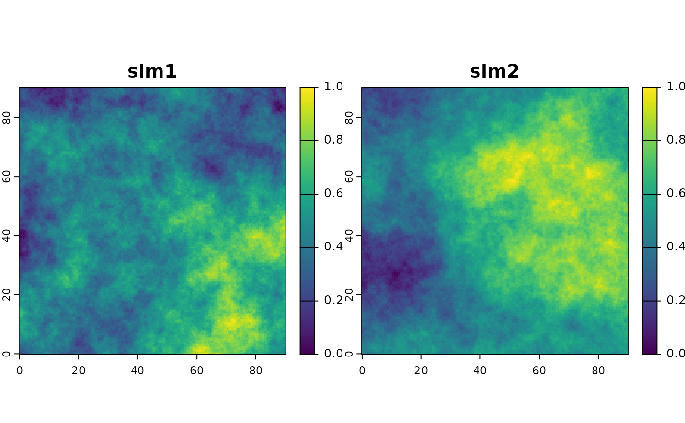

Build the suitability layer

The generate_resource_layer() function permits building a suitability layer from a set of environmental layers and beta parameters to be leveraged with. It mimics a basic resource selection function, where a given environmental layer is simply scaled by the beta parameter (env*beta) and several leveraged env layers are additively combined. For more elaborate procedures, see the virtualspecies package.

library(terra)
# simple example
grid <- create_grid()
cdt <- generate_env_layer(grid = grid)
#> [using unconditional Gaussian simulation]
rsce <- generate_resource_layer(env_layers = cdt$rasters,
                            beta = c(2, -1.5))
str(rsce)
#> List of 2
#>  $ dataframe:'data.frame':   32761 obs. of  3 variables:
#>   ..$ x          : num [1:32761] 0 0.5 1 1.5 2 2.5 3 3.5 4 4.5 ...
#>   ..$ y          : num [1:32761] 90 90 90 90 90 90 90 90 90 90 ...
#>   ..$ suitability: num [1:32761] 0.566 0.546 0.56 0.554 0.527 ...
#>  $ rasters  :S4 class 'SpatRaster' [package "terra"]
plot(rsce$rasters)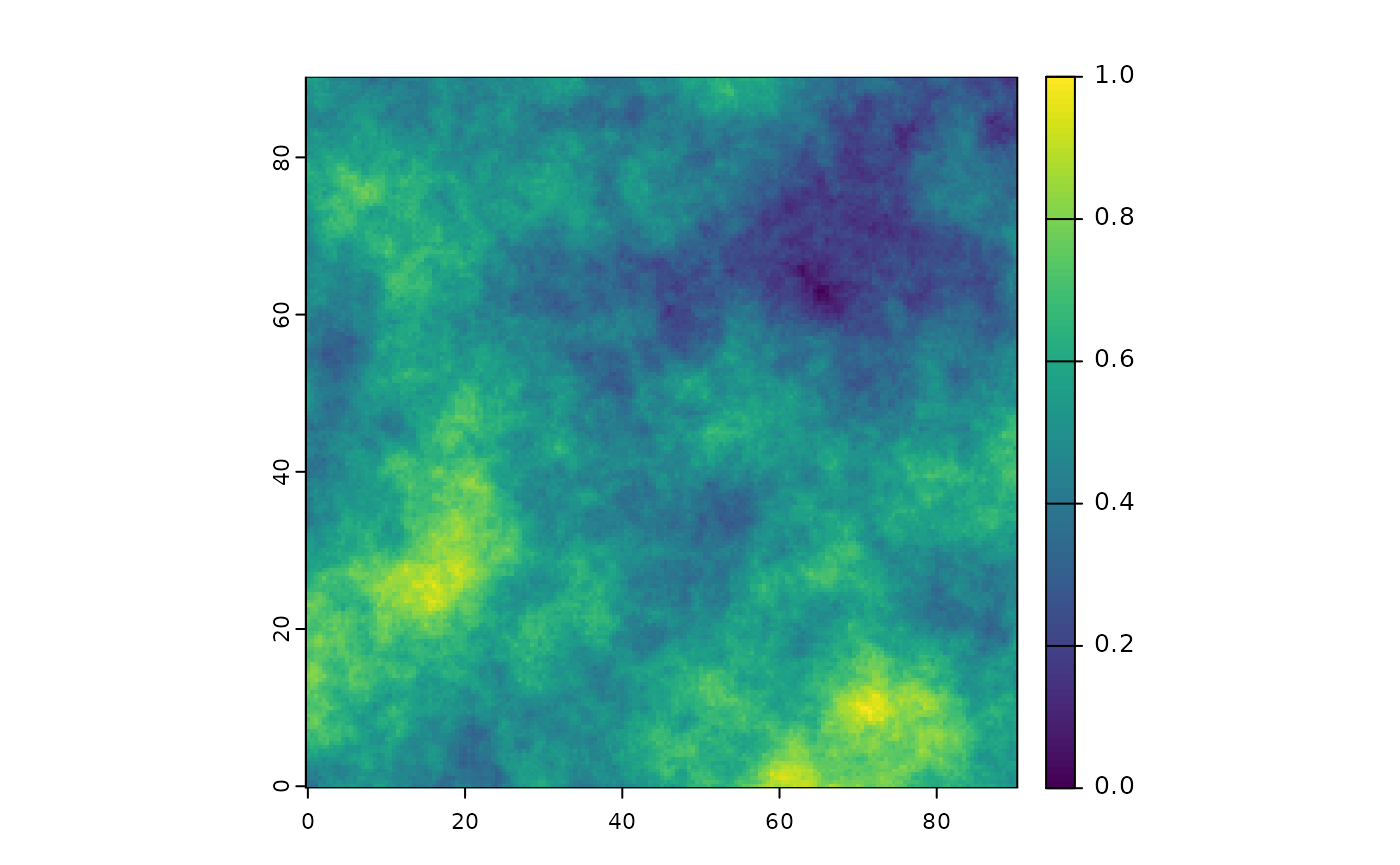


# also works when coordinates are not names x,y
cdt2 <- generate_env_layer(grid = grid, n = 3)$dataframe |> dplyr::rename(lon = x, lat = y)
#> [using unconditional Gaussian simulation]
str(generate_resource_layer(env_layers = cdt2, coordinate_fields = c("lon", "lat"),
                            beta = c(2, -1.5, 3)) )
#> List of 2
#>  $ dataframe:'data.frame':   32761 obs. of  3 variables:
#>   ..$ lon        : num [1:32761] 0 0.5 1 1.5 2 2.5 3 3.5 4 4.5 ...
#>   ..$ lat        : num [1:32761] 0 0 0 0 0 0 0 0 0 0 ...
#>   ..$ suitability: num [1:32761] 0.389 0.346 0.37 0.328 0.324 ...
#>  $ rasters  :S4 class 'SpatRaster' [package "terra"]